Metail Tech – Web, DevOps, 3D graphics, data engineering, systems, Clojure… y'know, that kind of thing

Colouring graphs for a wireframe shader

April 14, 2022 by David Gavilan·0 Comments

Various solid wireframe modes in Maya, Mesh Lab, and our WebGL Model Viewer (from left to right).

About solid wireframes

In order to spot problems in a mesh it is sometimes useful to look at the shape of its triangles or polygons. That’s what wireframe modes are for. But if there are too many lines it can be confusing to look at. That’s why it’s also useful in 3D CAD software to have a solid wireframe mode, that is, a mode where you only see front lines, and the rest are occluded by the triangles of the solid mesh. See the figure on top.

Because I use my WebGL Model Viewer to preview models quite often, I thought it would be a good idea to add a solid wireframe mode to it. Instead of attempting to draw actual line primitives, I thought it would be more fun to draw the lines directly from the triangles in a pixel shader. And that’s what I will describe in this blog post.

Barycentric coordinates

There’s a very easy way to know whether a point inside a triangle is at the edge of that triangle, i.e. the line we want to draw, or not. If we convert the coordinates of the point to barycentric coordinates, the point will be expressed as a 3D tuple (α, β, γ), where the 3 vertices of the triangle correspond to coordinates (1, 0, 0), (0, 1, 0), and (0, 0, 1). Any point where one of the coordinates is zero lies on one of the edges of the triangle. See illustration below.

In barycentric coordinates, one of the coordinates is zero for points in an edge

If we label each vertex with its equivalent barycentric coordinate, then the rasteriser can do the dirty work of computing the exact (α, β, γ) coordinates for every single pixel inside the triangle. Then, to draw white lines we can simply paint white pixels where one of the coordinates is zero, and paint black otherwise.

That works for a single triangle, but what happens when triangles share one or more vertices?

Graph colouring

In the triangle strip of the illustration below we need to assign barycentric coordinates in a way such that not two adjacent vertices share the same coordinate label. This problem is known as graph colouring in Graph Theory. The 3 barycentric at the vertices can be seen as 3 distinct colours, and then the question we want to answer is:

can we colour the graph (the mesh) with just 3 colours?

Barycentric coordinates on a triangle strip

Unfortunately the general answer to this question is NO. So, spoilers ahead, this shader I implemented doesn’t work for all meshes. But it turns out that many meshes are indeed 3-colourable. Let’s not get too deep into graph theory, but let’s check some examples instead.

Planar graphs are 4-colourable

The Four Colour Theorem states that a planar graph can be painted with no more than 4 colours. The proof of that is quite complicated, so let us just believe the result. However, it is NP-complete in complexity to decide whether an arbitrary planar map can be coloured with just three colours.

Moreover, 3D meshes aren’t planar graphs in general. A graph is planar if you can draw it on a plane without any 2 edges intersecting. I think this is related to the UV-unwrapping problem: if the graph is planar, you can unwrap the texture coordinates (UVs) of a mesh continuously on a plane, without having to break the UVs in pieces. Note that the opposite may not be true. For instance, in the examples below the cube isn’t planar, because no matter how we draw it, there will always be edges that cross. However, the UVs can be unwrapped on a plane, and it can be coloured with only 2 colours. On the other hand, the tetrahedron may seem not planar either, but if you draw it from above, its edges do not cross. So it’s planar, but it needs the maximum number of colours of a planar graph to be painted, 4.

The cube isn’t planar, but it’s 2-colorable. The tetrahedron is planar but 4-colorable.

Open quad strips are 2-colourable

Quads are used often for modelling. An open quad strip, as illustrated below, is 2-colourable. But quads are rarely supported by GPUs, so usually the quads need to be triangulated before rendering. By adding that extra edge, the new triangle strip becomes 3-colourable.

A 2-colourable quad strip, and a 3-colourable triangle strip

Quad strip loops are 3-colourable

If the quad strip “loops”, that is, if we close the strip so the mesh has a hole, we may need an extra colour to paint it. See below. If we triangulate that, we will need an extra colour, making the triangle strip loop 4-colourable.

A 3-colourable quad loop, and a 4-colourable triangle loop

Vertex colouring algorithms for meshes

It is NP-hard to compute the chromatic number of a graph, and the 3-colouring problem is still NP-complete on 4-regular planar graphs. But there are different algorithms we can use to colour a graph in polynomial time.

One of such algorithms is Gregory Chaitin‘s, which I implemented in the Model Viewer. If the mesh is 3-colourable, it seems to work well. However, it seems a more naive approach based on the inherent order of the vertices of the mesh works better for meshes that are not 3-colourable. See the examples below.

Graph colouring comparison through wireframes

Graph colouring comparison through wireframe. The left column uses Gregory Chaitin’s algorithm, whereas the right images follow the vertex ordering of the data.

In the example above, white areas appear white because 2 or more vertices share the same colour, so our wireframe shader that’s based in barycentric coordinates fails to paint just the edge. The mesh is not 3-colourable, so it can’t be helped. But, as it can be seen in the images on the right, we can do better if we paint the vertices in a different order. In this case, we simply follow the ordering given by the index number of the vertices in the mesh. The painting algorithm is simply:

For each triangle, sort its vertices by vertex index. E.g. [3, 0, 2] becomes [0, 2, 3].
Sort all the triangles in the mesh by “most significant” vertex index, i.e. we look at the first index of each triangle and if they are the same, we look at the next index. E.g. Given a = [2, 4, 20], b = [3, 4, 12], and c= [3, 5, 1], they will be sorted [a, b, c].
Then, for each triangle,
1. Start with 3 available labels/colours.
2. Remove vertices already painted, and labels already used by those vertices.
3. For the remaining vertices, assign the remaining labels in order. If we run out of available labels, the mesh may not be 3-colourable. Skip vertex.

That’s all.

The wireframe shader

It turns out that many meshes have a very regular structure and are indeed 3-colourable. So I thought it was still valuable to implement this shader, even if it doesn’t work for any arbitrary mesh. The shader is extremely simple:

vec4 lines = 1.0 / clamp(64.0 * vertexColor, 0.0001, 64.0);
float line = max(lines.r, max(lines.g, lines.b));
gl_FragColor = vec4(line, line, line, 1.0);

And the colours we paint the vertices with need to be exactly (1, 0, 0), (0, 1, 0), (0, 0, 1), because those represent the barycentric coordinates. The mixture of any other colours will make us to either lose one edge, or to paint the whole surface because some coordinate is non-zero. See some rasterisation examples below.

Rasterisation examples to illustrate the shader output given different vertex colours as input. Only pure Red, Green, Blue inputs result in a wireframed triangle.

The function that we use is an inverse distance function, scaled by some arbitrary number so we can make the lines thicker or thinner. Lines also get thicker as they get closer to the camera and the triangles get bigger. This is different from normal wireframe/line rendering, where the thickness of the line is always the same, regardless of the size of the triangles. You can see this effect in the image below, which also shows one of our models, that turns out to be 3-colourable.

Solid wireframe on a close-up of one of our models

In terms of implementation complexity, it was harder for me to enable vertex colouring than the actual shader. If you are curious, check this pull request: Model Viewer / Memory Layout. I refactored my old code so I could define the memory layout of the vertex data that I send to the GPU in a tidier way. I stored the colours as 32-bit RGBA values, so it’s just an extra 4 bytes per vertex.

Conclusion

This was a fun exercise to learn a bit about graph colouring, barycentric coordinates, and wireframe shaders, and how all those 3 things can relate together. Although the resulting rendering algorithm may create undesirable white patches in arbitrary geometries, it works for regular topologies like the ones in our models. Because lines are rendered using a distance function in a pixel shader, lines can look thick when you zoom in, an effect that may be desirable when you want to emphasise certain areas of the wireframe.

Skeletons & 3D File Formats: Why do developers create their own?

September 7, 2020 by David Gavilan·3 Comments

Why do developers create their own file formats?

The short answer is that existing standard file formats do not match the requirements of their applications. 3D file formats like COLLADA or glTF, for instance, are good for renderers, but not necessarily good for content creation software for artists. That’s probably why 3D modelling software like Blender and Autodesk Maya have developed their own file formats. Blender has .blend files, and Autodesk has developed FBX, a proprietary file format.

In this article I will be showing examples of both FBX and COLLADA (DAE files), but with a stronger focus on COLLADA for two reasons: 1) it has been around for a long time, so it’s widely supported by lots of modelling software and game engines (check the list in Wikipedia); 2) its specification hasn’t changed since 2008 (version 1.5), so one can assume pretty stable support across different software. FBX is also widely adopted, but applications like Blender don’t always support the latest version. Since FBX is a proprietary format, the best way to access it is through the FBX SDK, which gets updated every year. But that means constantly having to update your software. This variability may also be the reason why IEEE advocates for the use of X3D standard for “serious” applications (from a talk in 3DBody.Tech), although I don’t agree that stability equates with seriousness. Wavefront OBJ file format, for instance, is also very stable and widely used, but it doesn’t support skeletons, so that’s not an option in our application.

Although I’m going to be talking mostly about skeletons, similar challenges exist in other areas, such as the representation of geometry and materials.

About COLLADA and hints for problems

COLLADA was originally created by Sony Computer Entertainment and it is now the property of the Khronos Group, the people behind OpenGL and Vulkan. COLLADA defines an XML schema, so DAE files are in a human-readable format. Recent formats like glTF have moved away from XML in favour of JSON, which is a bit less verbose and still human-readable.

From my experience, the common compatibility problems with COLLADA files are around scale, orientation, and rotation order. Scale and orientation come from the metadata section (the asset node) at the beginning of the file:

<unit meter="0.01" name="cm"/>
<up_axis>Y_UP</up_axis>

Version 2 of the Open Asset Importer library (assimp), used by many other applications, did not have support for metadata so this information may be lost if your software is using an outdated library. Later versions do have support for it but still, after importing a COLLADA asset, the library converts the up axis to be Y_UP. In Blender, the default vertical axis is Z, so you can imagine that could be a source of confusion through imports and exports. Similarly with scale, much software does not apply that global scale to the scene, so your objects may look gigantic if the units are in centimetres and your engine default unit is metres.

The other big source of confusion seems to be around rotation orders. COLLADA can represent rotations using matrices, or using an axis-angle. For instance, a 90-degree rotation along the Y axis can be written as:

<rotate>0 1 0 90</rotate>

If you concatenate rotations, they need to be applied in the inverse order in which they appear in the XML document. Depending on the XML parser you are using, it may be difficult to extract this order, since it’s not an attribute of any of the nodes. For instance, to rotate 90 degrees along Z and then 90 degrees along X we can write:

<rotate sid="rotateX">1 0 0 90</rotate>
<rotate sid="rotateY">0 1 0 0</rotate>
<rotate sid="rotateZ">0 0 1 90</rotate>

To convert to and from axis-angle representation and Euler angles we need to remember this rotation order. The above can be written as a (90, 0, 90) Euler rotation with XYZ rotation order. If we flip the rotation order to be ZYX we would obtain a very different result, as illustrated in the example below.

The order in which rotations are applied greatly affects the result. Here Z is the vertical axis, and X the horizontal.

If your application only cares about rendering the final object on screen, it could be correctly reading rotation nodes and then converting them to matrices, since that is all that is needed to display things. But you may not be able to obtain an Euler-angle representation if it doesn’t store the rotation order somewhere.

Skeletons: bones and joints

In a previous blog post, Introduction to skinning and 3D animation, I briefly introduced the difference between a bone and a joint. Let’s read this quote from the COLLADA specification 1.5.0 (page 37):

Skinning is a technique for deforming geometry by linearly weighting vertices to a set of transformations, represented by <node> elements. Nodes that affect a particular geometry are usually organized into a single hierarchy called a “skeleton,” although the influencing nodes may come from unrelated parts of the hierarchy. The nodes of such a hierarchy represents the “joints” of the skeleton, which should not be confused with the “bones,” which are the imaginary line segments connecting two joints.

Joints define a space transform, which can be represented by a single matrix. As I mentioned in the previous section, this is all we need for rendering, but an artist may find other attributes useful for easier manipulation. For instance, a bone as defined in Blender has a roll that can not be inferred just from the joint matrices without some assumptions. The 3D authoring software could have some physical rotation limits to avoid rotating a joint more than is physically possible, like in the DazStudio screenshot below. Those constraints do not get exported to COLLADA, so if you use DazStudio to export an avatar to COLLADA and import it back, those constraints will be lost.

Bone attributes in Blender (left) and joint rotation constraints in DazStudio (right). The red, green, and blue circles show the available rotation range.

As I hinted with the DazStudio example, some software is not capable of correctly importing the file that is exported, and this is not always a limitation of the format you export to. I will show you some examples in the next section.

Real skeleton import/export failures

Asset preparation

I am going to show you some funny bugs in this section. I’m going to focus on poses gone wrong because of bad rotations, although in some of the examples the scale went wrong as well and I had to manually adjust the scale so that everything uses the same units.

In all these examples I’m going to use a model from DazStudio as an input. The model has several keyframes with different poses, and I’ll be showing the first pose where the avatar has his head facing to his left, and his left leg bent towards his right, behind his right leg. See below:

Model and pose created in DazStudio, used in the experiments.

Once exported to COLLADA, I’ve verified that the scale and axis in metadata looks correct:

    <unit meter="0.0099999997" name="cm"/>
    <up_axis>Y_UP</up_axis>

The exported rig has the peculiarity that it contains no rotations, i.e. it’s all expressed in a global axis. This is a bit strange, because expressing twists won’t be straightforward if the axis of rotation doesn’t follow the direction of the bone, but having no rotations makes things simpler in our tools. The rig only contains the position of the joints, and the rotation order expressed as a list of axis-angle rotations with 0-angle rotations. For example, the hip joint node looks like this:

<node id="hip" name="hip" sid="hip" type="JOINT">
  <translate sid="translation">0 103.6847992 -0.1028240994</translate>
  <rotate sid="rotateX">1 0 0 0</rotate>
  <rotate sid="rotateZ">0 0 1 0</rotate>
  <rotate sid="rotateY">0 1 0 0</rotate>
  <scale>1 1 1</scale>
  <node id="pelvis" ...>...</node>
  <node id="abdomen" ...>...</node>
</node>

So the rotation order for the hip XZY. Because Y is the vertical axis, that means that you first decide where to face when rotating the avatar, i.e. a rotation along Y. That makes sense. Let’s hope all software understands that order when reading the angles from the poses.

Apart from DazStudio, I’m going to use the following software and several conversions between them and see what happens:

Blender 2.83.3, for visualisation (import) and exports;
Autodesk Maya 2020.2, for visualisation;
FBX SDK 2019 (used in our internal tools), for exports;
assimp 4.0.1 library (used in our internal tools), for imports;
My WebGL Model Viewer, for visualisation of COLLADA files only. This viewer only cares about rendering, an easier job than trying to reconstruct bones from joints, as explained earlier.

DazStudio export

Using DazStudio exporters, I’ve exported the Daz3D model to DAE and to FBX. This is what the FBX file looks like in Blender and Maya:

DazStudio model exported to FBX, and opened in Blender and Maya.

The bones look the right size in Blender, but the rotations and translations went all crazy. The rotations are correct in Maya, but the bones are just lines connecting joints. Let’s see what happens if we use DazStudio to export the same file to DAE:

DazStudio model exported to DAE, and opened in Blender and Maya.

The bones are now the right size in Maya, but the rotations are still wrong in Blender. The bones in Blender are now tiny, and still pointing up. I suspect they point up because the rig contains no rotations, as I mentioned in the previous section.

FBX-SDK import & export

Let’s experiment with the FBXImporter and FBXExporter functions from the FBX-SDK. This is the FBX that comes from reading the DAE file that DazStudio has created:

DazStudio DAE model exported to FBX using FBX-SDK.

The FBX file in Maya looks OK, and the FBX file looks slightly better now in Blender than it did when directly exported from DazStudio, although the rotations are still wrong. Let’s try reading the FBX file that DazStudio created, and exporting it to DAE with the FBX-SDK:

DazStudio FBX model exported to DAE using FBX-SDK.

The file still looks fine in Maya, but Blender fails to read the file. In the Model Viewer, the pose looks correct, but the normals have gone funny at the boundaries of the submeshes — that’s why there are black lines in those areas (not too important, since we can recompute the normals). A bit more worrying is that the names of all joints have changed, which is not ideal. For instance, the hip becomes hip_ncl1_1.

Assimp for import & FBX-SDK for export

Here we are using our own tools. We use the assimp library for importing the DAE file created with DazStudio, convert it to our internal model format, and then use the FBX-SDK to create a new FBX file. That FBX file looks like this:

DazStudio DAE model exported to FBX using assimp for import and FBX-SDK for export.

Finally the pose looks right in Blender. The bones are all pointing upwards, but at least they now look the right size. You can try to fix the bones in Blender by manually connecting the tail of each bone to the head of the next bone. However, the roll of the bones is wrong. There’s an option in Blender to compute the rolls automatically for you, but for some reason the roll becomes 57 degrees. I don’t understand why a roll of zero does not face any of the major axes.

Maya looks fine. Let’s use the FBX-SDK to save our model as DAE:

DazStudio DAE model exported to DAE using assimp for import and FBX-SDK for export.

The pose still looks fine in Blender, although the bones look tiny this time. Maya still looks fine. We could stop here because this seems to be the best we can get, but let’s do a final test.

Blender export to DAE

Let’s see how the COLLADA exporter in Blender behaves. If we load the FBX model exported from our tools, which looked OK in Blender, and save it to DAE, we get this new file:

FBX model from our tools exported to DAE using Blender.

Inspecting the metadata, the scale is now 1 metre units and the up axis has changed to Z_UP. The original file had Y_UP and centimetres (0.01) for the scale. In the Model Viewer and in Maya, the armature/rig got disconnected from the mesh. It seems that the names of joints in the animations have been prepended with the name of the root node, whereas the names of joints in the rig have stayed the same. So the keyframes get ignored and you can only see the binding pose, i.e. the T-pose. Blender must know something of what it’s doing, because the keyframes are still there, but totally broken.

Now let’s read the DAE file and save it again as DAE from Blender. It’s not the identity operation as one might expect:

DAE model from our tools exported to DAE using Blender.

We have the same problems as before with the scale and disconnected armature, but the keyframes are also lost to Blender this time. The vertex normals went a bit funny, that’s why the surface doesn’t look smooth anymore.

Our parsers and formats

From the failures above you can see that what works best for us is exporting the DazStudio file to DAE, and then using the assimp library to convert it to our internal format. The assimp library can’t be greater than version 4, though, because in version 5 the XML library that they use to read DAE files throws an exception. The newest version fails to read empty XML entities such as <author/>. I recommend writing unit tests for any external libraries that you use. These unit tests just need to exercise the parts of their API that you use, but this way it will save you headaches when you attempt to update to a newer version.

For the Model Viewer I wrote my own parser so I could keep adding support for every strange case I encountered. That’s why in most of the cases I presented earlier the poses look fine in the Model Viewer. I could probably even add support for the last disaster that Blender creates, because inspecting the file in plain text I can see where things went wrong. However, if not even Blender can read the mess it has created, it feels pointless to add support for such messy DAE files.

So why don’t we just keep all our model files in COLLADA format? Poses in DAE or FBX files are stored as keyframes in an animation, with no possibility to name the poses. For our purposes, we describe poses as a series of joint rotations, with a label associated to each pose. We decouple translations and scale from joints and store them separately to describe a body shape. We also store other things such as the angle rotation constraints that you can see in DazStudio. This is what I referred to in the introduction when I said that existing file formats may not match the requirements of your application.

Conclusions

There is no magic formula to solve the compatibility problems with rigged 3D models. Developers will continue to create custom formats for their applications because requirements change from application to application. If you can do everything with Blender, then stick to their format. However, never use Blender to export COLLADA files because their exporter is a total mess. The COLLADA specification has been around for a long time and it does look quite straightforward, so one might expect better compatibility. But that’s rarely the case. I wouldn’t get too excited by new formats like glTF because reading the glTF 2.0 specification on Skins and Animations, they look basically the same as COLLADA but in JSON format. This is not a surprise, because that’s what you need for rendering, but modelling software needs more than that.

Autodesk Maya is more robust than Blender when importing skeletal models from different sources. Maya is not free, though. if you just need to read or write FBX files, you can get their FBX-SDK for free. For reading COLLADA files I would use assimp, though, because the FBX-SDK changes the name of the joints and introduces some other artefacts, like messing up the normals.

Finally, just a reminder that we are already in 2020, in case you thought I was writing this in the late 90s. 🤷‍♂️

The Stencil Buffer and how to use it to visualize volume intersections

July 3, 2020 by David Gavilan·0 Comments

Visualization of Volume Intersections

Introduction

The trendy thing in real-time rendering these days is ray-tracing. However, traditional rasterization hasn’t disappeared, and it won’t in the near future. I recommend this blog post on the subject: A hybrid rendering pipeline for realtime rendering: (When) is raytracing worth it?

I find that one of the most neglected elements in the rasterization pipeline is the Stencil Buffer. To get an idea of how neglected it is, I’ve checked the number of appearances of the stencil buffer in the approximately 1000 pages of “Real-Time Rendering”[1]: it appears just 5 times, and there are no more than 4 paragraphs dedicated to it. At least for me, it’s hard to get my head around the stencil buffer because it’s not fully programmable, so I tend to avoid using it. You can only configure it, and to do so you have to think of Boolean algebra, but in 3D.

This blog post is an attempt to demystify the stencil buffer. I will briefly review the rendering pipeline, to see where the stencil sits, and then explain how the stencil works. I will use an example application in WebGL that we use to detect volume intersections, and explain the steps to convert the algorithm in my head to a tabular format that can be used to configure the stencil.

The Rasterization Rendering Pipeline

Rasterization Rendering Pipeline in the GPU. Some stages are fully programmable, others are configurable, and others are completely fixed.

Virtually every GPU implements a rendering pipeline like the one above. In the middle row I tried to illustrate the transformations that we apply to our models until they become an image on the screen. In the vertex shader, we receive the triangles that make up the surface of our 3D model. Then, our vertex shader will apply a series of matrix multiplications to those triangles to convert from the model space (origin of coordinates centered around the model), to world space (origin of coordinates in the world origin), and then to camera space (origin of coordinates in the camera). Then, we apply a projection transform (perspective or orthographic), so the camera frustum becomes a unit cube. Whatever is outside that unit cube gets clipped, and mapped to screen coordinates. Then the rasterizer converts those triangles into pixels, interpolating color values between vertices. Then we can apply operations per pixel in our pixel shader, and blend the result into the frame buffer that we see on screen, in the merger stage.

The merger stage: blending, Z-buffer, and stencil

That merger stage does mainly 2 types of operations: blending and discarding pixels. The blending, or Alpha Blending, blends pixel colors of our object with the colors already in the frame buffer based on the alpha value of the texture of the object. The alpha value is typically 8-bit, so there are only 256 possible values. We can also use the alpha value to discard pixels as well, based on a threshold. Pixels with a value smaller than the threshold will be discarded. That’s referred to as alpha masking.

Pixels can also be discarded thanks to the Z-buffer. The Z-buffer contains the distance (Z) from the camera to the objects in the scene. Say we have rendered the mountain from the illustration above, and now we try to render a tree that’s behind the mountain. The Z-buffer contains the distance to the camera for every pixel of the mountain. We can compare the Z values of the tree, and discard them if the new Z value is greater than the Z we have already. The tree won’t render. Notice that if we change the rendering order and render the tree first, it will get rendered. However, once we draw the mountain the Z-test won’t fail, so the mountain will be rendered on top. So some pixels will be drawn over several times. That’s what we call the overdraw, which can be used to measure efficiency. Sorting the scene is a way of reducing the overdraw.

Lastly, we can use the stencil buffer to discard pixels as well. The stencil buffer is typically an 8-bit buffer, so 256 distinct values are possible. In its simplest form, it can be used as an alpha mask. Say that we are seeing the mountain through a window, and we want to hide everything else. We can mark the pixels that belong to the window with an arbitrary number in the stencil buffer, e.g. a 1 signifies a pixel from the window, and then we configure the stencil buffer to discard everything that it’s not labeled as “window”. When combined with the Z-buffer, the stencil buffer can be used as a powerful tool to create volumetric effects, as we will see in the example later on.

Stencil buffer configuration

To configure the stencil buffer we have 3 types of settings:

Comparison functions. This is the function used to decide whether to discard a pixel or not. For instance, “greater than”, or “less than”. See: available stencil functions in WebGL.
Mask values. These are 8-bit binary masks. There are 3 types of masks: reference, read mask, and write mask. In WebGL, the reference and read mask are set with the stencil function, whereas the write mask is set with the stencil mask. The reference and read mask are used in conjunction with the comparison function. For instance, if the comparison is set to “greater than”, the stencil test will pass if (refMask & readMask) > (stencil & readMask), where “&” is a bitwise binary AND operation. The write mask gets applied to what we write to the stencil buffer if the test passes and we decide to update it.
Stencil operations. These are actions that can be configured in case of a successful or a failed test. You can do things like keep the current stencil value, replace it, or increment it. See: available stencil ops in WebGL. The actions can be configured for the 3 following conditions:
- fail: the stencil test fails
- z-fail: the z-test fails (see Z-buffer in previous section)
- z-pass: both the stencil and the z-test pass.

Writing it down as one big logical operation, for each pixel, the new value of the stencil buffer can be computed as follows:

if (refMask & readMask) Comparison (stencil & readMask): 
    stencil_new = (stencil & ~writeMask) | (writeMask & Operation(stencil))

It does sound very abstract, doesn’t it? How do all these logical operations become something useful? I hope with the example in the next section you learn how to configure the stencil.

Visualizing volume intersections with the stencil buffer

Visualization of cube intersections and back faces

Problem definition

Let start with the problem definition. We want to visualize the volume intersections in a mesh, and any open areas of the mesh. This is a quick way of visually detecting if a mesh is watertight, i.e. the mesh contains no holes and it’s clearly defined inside. Holes are easy to visualize if we render the object in 2 passes. A vertex has 2 sides, front and back. Whether a side is front or back is decided by an arbitrary vertex winding order (it can be configured). When rendering, back faces are usually not rendered, but this culling is one of those things that can be configured in the render pipeline. So we can do a first pass where we render only the back faces in a bright green color, and then a normal pass where we render the rest. If we see green on screen that means that the mesh has a hole in there.

Configuration for volume intersection

For the volume intersection things get a bit more complicated. I know that the stencil should be useful in this, but how do we set it up? I always start writing down on the white board all the examples of triangle layerings that I can think of. Then, I know that in the end I want a stencil mask that marks exactly the intersection area in the given example. What operations can take me there? There are multiple. The challenge is to find one that works for all the examples you’ve written down. There must be a better way to draw this, but this is what I got:

Stencil Configuration by Example. We are trying to figure out a way to create mask for areas of volume intersections.

Then, once I think I have all the cases I need, I try to fill in a table with all the stencil configuration per render pass. From the picture above, you can see that the way I designed it, I’m going to need at least 3 passes:

one to render the back faces, where I count the number of back-facing polygons;
a second pass to render the front faces and decrease the counter if the z-test fails. We will avoid writing onto the Z-buffer so we can distinguish those 2 circled cases (where front-face B is rendered before front-face A). Because during the back pass we update the Z-buffer, the Z-buffer before starting the 2nd pass contains the z value of the back face closer to the camera. In the non-intersecting example, the order doesn’t matter, because whether the Z-buffer contains the z of the back-face or the z of B, we can detect a z-test failure when trying to draw A and decrease the counter. But in the intersecting example, if we draw face B first and update the Z-buffer, when trying to draw face A the z-test will fail and we will wrongly decrease the counter. To solve this without having to sort the geometry, we will stop all Z-buffer updates (Z-write off) during this pass.
a third pass to create a binary mask with the intersection area.
I can add an optional 4th pass to render the lighting of the non-intersecting volumes.

Here’s my final stencil table:

Pass	Func	Ref	Read Mask	Write Mask	Fail?	Z-fail?	Pass?	Z-write
Back	ALWAYS	`0`	`0`	`0xf~f`	KEEP	INCR	INCR	ON
Front	ALWAYS	`0`	`0`	`0xf~f`	KEEP	DECR	KEEP	OFF
Front – intersection	LESS	`0x1`	`0xf~f`	`0xf~f`	KEEP	KEEP	KEEP	ON
Front – light	GEQUAL	`0x1`	`0xf~f`	`0xf~f`	KEEP	KEEP	KEEP	ON

If you want to check how that translates into code, check this pull request in GitHub: self-intersections for WebGL Model Viewer.

Visualization results

Here’s a video of the WebGL Model Viewer in action:

The green areas are back faces, so holes in the mesh, whereas the red areas are the volume intersections. One application of this is to help us spot issues in poses in our avatars. If part of the arm intersects with the chest, we will have problems when trying to dress the avatar with a shirt, because the sleeve will also try to enter the chest and the cloth simulation will struggle. See example below:

Volume intersections and cloth simulation

The visualization of volume intersections (middle) can warn us about future problems in cloth simulation (right).

Conclusion

Rasterization is still the most used rendering pipeline in real time graphics. Inside the rasterizer, the Stencil Buffer seems to be the ugly duckling no one wants to hang around with, perhaps only reserved to big graphic gurus. I have showed you with a practical example that we can use the stencil buffer to visualize volume intersections in real time, and that the stencil is not as scary if we describe the problem with examples and in tabular form.

Visualizing volume intersections in real time has a practical application for us. When we author poses for our avatars, we can immediately see if a pose will end up having cloth simulation problems, and correct the limb position accordingly.

For more applications of the stencil buffer, check the “Real-Time Rendering” book [1], and the Wikipedia article.

References

[1] Tomas Akenine-Möller, Eric Haines, Naty Hoffman. Real-Time Rendering, Third Edition. A K Peters, 2008.

What’s wrong with that pixel? The backward journey of light

May 26, 2020 by David Gavilan·0 Comments

Introduction

When we take a photograph outside, we are capturing light that has travelled 150 million Kilometres (1 au), scattered in the atmosphere, bounced on an object, to finally be captured by the camera sensor and stored as numbers in an image file. The rendering process in Computer Graphics is basically the same, but the world happens to be virtual, so the image numbers come from a simulation inside the computer.

There are many publications and books on Computer Graphics and it can be overwhelming at times for people who want an introduction to rendering & imaging. Most books explain how light gets transformed until it gets synthesised into an image. In this article, though, I’ve tried to do the journey backwards, to help people troubleshoot the possible things that have gone wrong when they feel a pixel in the screen looks funny or the wrong colour. You can follow the journey with me, or you can skip directly to some practical tips I list up in the last section.

Your eyes: the end of the journey

Whatever image we produce, ultimately is going to be consumed by human eyes. And what I perceive may not necessarily be the same as what you perceive. Perception is a psychological process that includes sensation, memory, and thought and results in meaning such as recognition, identification and understanding [1]. What a person sees and experiences is called a percept (the product of perception, which is a process). What a person reports seeing is a verbal attempt to describe a nonverbal experience.

I’m not going to discuss visual perception in detail, but I’ve started the discussion with this because more often than not problems with images are simply a mismatch of expectations. Specially if all the communication, from a person requesting an image to the final evaluation, has been verbal. Let’s use the famous Adelson’s checker shadow illusion as an illustration:

The squares marked A and B are the same shade of gray.

Because our brain reconstructs the 3D scene it’s seeing, it knows that square B is lighter than square A. But in terms of pixels, both A and B have exactly the same shade. You can verify this by using a finger to connect both squares. Knowing this, you can recognise this request as ambiguous: “could you make B brighter?”. There are many ways to achieve that, all with very different results: paint B brighter, making it stand out; increase the overall exposure of the image, making A also brighter; add a spot light directed towards B making it and its surroundings brighter, and so on. If you want to see more of these visual tricks, I recommend you the book Mind Hacks [2].

What are the colours of shadows?

As seen with that example, a common misunderstanding in communication is mixing up the brightness of an object with the brightness of the light. This applies to colour as well. If I ask you for the colour of a shadow outdoors, would you say it’s grey, blue, or the colour of the object where it’s projected, e.g., green if on grass? In terms of pixel values, shadows outdoors are blueish, because that’s the colour of the ambient light that comes from the sky. This is also the reason why it is preferable to sketch drawings using a blue pencil if you are going to colour the drawing later. But many won’t explicitly perceive those shadows as being blue.

A dot in a screen

Let’s assume that the image you are seeing is in a screen, although similar discussions will apply to printed form. Many things can go wrong when displaying an image on a screen:

different monitors have different colour gamuts;
depending on the technology, the brightness of a pixel can affect the brightness of the pixel next to it;
even when using the same model of a screen, users can have different colour temperature settings, automatic time-of-day adjustments, colour filters, or even physical screen filters.

Warmer colours by decreasing the colour temperature

The correct thing to do would be that all parties use a colorimeter to calibrate their monitors, but more often than not colour calibration is only a must for people digitising the world, e.g., to make sure a material they photograph appears the same on screen. For other people I often recommend they download the image into their iPhones or iPads. This has the advantage that it’s a well-known screen, and it should look the same for everyone, provided that they don’t have any screen filter and that they have disabled the Night Shift. Recent smartphones screens use OLED displays, which do not suffer from brightness bleeding, and provide a wider colour gamut, Display P3 on Apple devices. Apple software also tends to do the right thing with the image, that is, they handle colour profiles correctly. Which brings us to the next topic.

Pixels in a file

Mainly 3 things can go wrong when displaying an image from a file: wrong colour profile, quantisation artefacts, and encoding artefacts.

Colour profiles

Comparison of some RGB and CMYK colour gamuts on a CIE 1931 xy chromaticity diagram. Source: Wikipedia

A colour profile describes the colour attributes of a particular device, and how to map between different colour spaces. I recommend reading a previous article where I introduced the concept of colour spaces. But for now just bear in mind that if different screens have different gamuts and different colour capabilities, we would need a way to convert between them, without losing information whenever possible.

Errors here can happen when saving the file, and when displaying it. When saving the file, we could working with a particular colour profile, e.g. Adobe RGB, and then forget to embed the profile in the file that we save. Or the format that we choose as output does not accept colour profiles. Then, the software displaying that image will assume a default colour profile, which it’s usually sRGB. Colour will look wrong. But even if we do embed the colour profile, not all software process it correctly. For instance, some browsers assume PNG images are always sRGB, and ignore their embedded colour profile. And yet again, even if the software does understand colour profiles, we need a rule to convert from one space to another, the render intent. The default may not be what we expect. In the example below, I loaded an image in sRGB colour space (the right image) into Photoshop (left image). Photoshop has converted the colour space to Adobe RGB. To make things more complicated, I have then taken a screenshot of Photoshop and the original image in macOS Image Preview, and what the screenshot does is storing the colour profile of my monitor in the resulting image. The important thing to notice is the colour shift that happens in Photoshop:

sRGB image loaded into Photoshop has its colours shifted by default. Drawing generated with AI Gahaku.

In the previous post, I also give some testing images in Display P3 colour space. In general, for images on the web I recommend sticking to sRGB, unless we are specifically targeting Apple devices, where we could use Display P3 to make use of the wider gamut.

Another word of warning is the common practice of taking screenshots. When you take a screenshot, at least with the default tool on macOS, it embeds the colour profile of the screen where you took the screenshot, Display P3 in many cases. Say you drag&drop that screenshot to some online slides. The screenshot could be wrongly read as if it were in sRGB, and the colours would look wrong. If the original thing we wanted to embed was in sRGB, it would have been better to drag that image instead of the screenshot.

Quantisation artefacts

Quantisation is needed to convert a continuous signal into a discrete one. Most of the images we see online use 8 bits per colour channel, which means only 256 distinct values. When using three colour channels, like in RGB colour spaces, that would make for a total 16 million colours when combined. It sounds like a lot, specially considering that the human eye can distinguish just up to 10 million colours, but it’s not enough to cover gamuts wider than sRGB.

To avoid quantisation problems, we need to store images with more bits per channel. PNG images in Display P3 will use 16 bits per channel. Without considering the alpha channel, that’s a file up to 3 times bigger. For instance, the image below was originally a 295KB 16-bit PNG image in Display P3 colour space. I have converted to a normal sRGB image, with 8-bits per channel, and the PNG size became 75 KB. In comparison, the image to the right only uses a 256-colour palette, and occupies 25 KB on disk.

8-bit sRGB (left) vs 256-colour palette (right). Image generated with Palettist.

Quantisation artefacts usually translate into banding artefacts. These banding artefacts are more visible in changes of luminance than in changes of colour, though. The quantisation I did with the image above when I converted it to 8-bit has introduced some banding, although it is probably hard to notice. The 256-colour image to the right should help illustrate the banding that occurs when you don’t have enough colours.

High Dynamic Range (HDR) images also require more bits per pixel in order to store a wider luminance range. Because most screens have a limited luminance range, HDR images have to be tone-mapped into Low-Dynamic Range before displaying. That could simply imply selecting the exposure, or applying some artistic post-processing. Most HDR TVs use a 10-bit encoding for encoding both a higher luminance range and a wider RGB gamut. TVs then come with a series of preset filters that tone-map the signal in different ways. But if the assets in a game are not HDR-ready, no matter that your HDR-ready Playstation 4 is connected to an HDR TV, you may still see some banding artefacts.

Encoding artefacts

This is probably the easier problem to spot and the easier problem to solve. Images would be very big if stored as raw pixels. On a 4K TV, images are 4096 × 2160 pixels. If we use 16-bit RGB images, the raw size will be 4096 × 2160 pixels × 6 bytes/pixels, approximately 50 MB for a single image. But images contain lots of redundancy, both spatially and in frequency, so fortunately we can compress them.

The most common formats on the web are still PNGs and JPEGs. PNG images use lossless data compression, so the resulting images are still a bit big. JPEG compresses much more, but it suffers from the block artefacts characteristic of the Discrete Cosine Transform (DCT). JPEG was supposed to be replaced by the JPEG 2000 (JP2) standard, which uses wavelet transforms to compress not only in the frequency domain as the DCT, but also in the spatial domain. It produces much better quality images for the same level of compression, and it also supports alpha blending, but unfortunately it is only supported widely in Apple devices. Recent browsers also support WebP, which uses DCT and entropy encoding. Not for the web, but also worth mentioning Open EXR, a format created by ILM that supports 32-bit HDR images, so often used as the preferred output of ray-tracers and renderers.

Below I’ve put some examples of the types of artefacts you will see if someone compresses the image too much using JPEG. Since we can’t recover what’s already lost, the only solution is asking the person who exported the file to export it again with better quality, or with lossless compression.

Illustration of block artefacts in JPEG

Light before turning into pixels

It’s time to get physical. Let’s assume we have a virtual 3D scene in our computer. That scene contains a series of objects, that is, geometry with materials assigned to them, a bunch of lights, and a virtual camera. Let’s discuss what needs to happen for it to become an image.

I’m going to cover mostly some equations on radiometry, the field that studies the measurement of electromagnetic radiation. For light, that radiation is the flow of photons, which can behave as particles or waves. The wave behaviour can mostly be ignored in rendering. Photometry studies similar things, but it weights everything by the sensitivity of the human eye. So even though most equations come from radiometry, many application use photometry units. The last important field is colorimetry, the field that tries to quantify how humans perceive light. The article about colour spaces gives more details. Here we just need to know that we can divide light into three separate signals, what we call the red, green, and blue channels, and that the equations presented here can be applied to each channel independently. I’ve tried to summarise here the most important things of the Advanced Shading and Global Illumination chapters in Real-Time Rendering [3].

The shading equation

The image that we see is a series of discrete values captured by a camera sensor, whether a real sensor or a virtual one from our renderer. The value captured by the sensor is called radiance (L), and it’s the density of light flow per area and per incoming direction. Here’s a quite complete shading shading equation used to compute radiance:

Eq. 1. Shading equation

It looks complicated, but it’s a quite straightforward sum of all the lights in the scene, because irradiance E is additive. The irradiance is the sum of the photons passing through the surface in one second. The units of the irradiance are watts per squared meter, equivalent to illuminance in photometry, measured in lux. Radiance is measured in watts per squared meter and steradian, equivalent to luminance in photometry, measured in nits, or candelas per squared meter. Let me roughly explain the terms in equation (1):

L_o is the outgoing radiance, which depends on the view direction v.
The first term adds the contribution from the ambient light. In an outdoor scene, that would be the sky. K_A is an ambient occlusion term, and c_amb is a blend of the diffuse and specular colours of the material. E_ind is the irradiance of the indirect light, which can be a constant. ⨂ is the piecewise vector multiplication.
The number of light sources is n, and l_k is the direction of the k-th light source.
υ (upsilon) is a visibility function, which corresponds to shadows for direct light sources.
f is the Bidirectional Reflectance Distribution Function (BRDF). It describes how light is reflected from a surface given the incoming light direction l and outgoing view direction v.
The final term is the irradiance of each light multiplied by the clamped cosine of the angle between the light and the surface normal. That means that if the surface is perpendicular to the light (the normal is parallel to the light), the surface will be fully lit, and in shade otherwise. The cosine is clamped because negative values are light below the surface.

Angle between light direction and surface normal

Let’s look at the BRDF as well. For most rendering needs, we can use the following equation:

Eq. 2. Blinn-Phong BRDF extended to include Fresnel

This is the Blinn-Phong model, extended to include a Fresnel term. The terms are:

c_diff is the diffuse colour of the surface, the main colour that we will see in non-metallic objects.
The next term is the specular light, very important in metals, but also present in most materials. m is the surface smoothness, and h is the half vector between l and v.
R_F is the Fresnel reflectance, responsible of the increase of reflectance at glancing angles. It’s usually approximated by the Schlick approximation, an interpolation between white and the colour it would be when the light is perpendicular to the surface (i.e. when alpha is zero).

Again, all this looks complicated, but in practical terms what it means is that we will have a series of RGB values that can be arbitrarily big to represent the irradiance, that will get multiplied by RGB values normalised from 0 to 1 that represent the colour of the surface and the presence or not of shadow. Then, we will add all these values together. I wanted to put all the terms in here because if you understand what each term means, it can be easy to troubleshoot problems in the rendered image. For instance,

if all the shadows look completely black, we have probably forgotten to add the ambient term, which in turn could mean we forgot to add an environment map (see next section).
If the object looks all black, but you can see highlights, it could mean that c_diff is zero, so perhaps what you are missing is the albedo map (see next section).
If the object looks too metallic, the specular term is to blame, so you need to check your material settings.
If there is lack of contrast between lit surfaces and parts in shadow, it probably means that your lights are not strong enough.
If your scene is outdoors but colours on objects do not look warm, perhaps the irradiance is monochromatic. If you are using an environment map, it could mean that the sun saturated to white when photographed. Did you capture light correctly?

Examples of unexpected material appearance. Garment created with VStitcher, and rendered with V-Ray.

Rendering techniques

Light doesn’t just travel from the light source to the object surface and then to the sensor, but it bounces around. Most real-time rendering methods use “tricks” or approximations to model global illumination. For instance, you can render the scene as if seen from the light to compute something called a depth map, and use that when you are rendering the scene from the main camera to figure out if a pixel is in shadow or not, that is, the value of the visibility function. There are many artefacts in real-time rendering, depending on the rendering engine that we are using: lack of soft shadows, jaggies in shadows, monochromatic ambient occlusion, lack of texture in clothes, and lack of material correctness in general.

Ray tracing is often used as the ground truth to see what a scene should look like. It is also used to “bake” or precompute textures that will be used in real-time renderers. Modern GPUs have some hardware capabilities to do ray tracing in real time, but it is still quite computationally expensive. Note that ray tracers do not usually follow the journey of light from the light source to the camera. Instead, as in this article, the journey of photons is followed backwards. It is way cheaper to project rays from the camera onto the scene, since we aren’t interested in rays that do not end up on the screen (or sensor).

Ray tracing has its own artefacts, mostly related to the quality settings of the ray trace. These are usually easy to spot. Because we can’t sample rays in every direction (because there are infinite), we need to quantise the number of directions we sample. That means using some kind of stochastic sampling of a sphere, like the Monte Carlo method. If there are not enough samples, there will be a distinctive noise in the images that looks like peppered shadows. When similar techniques are applied to real-time rendering methods, the number of samples is even lower, but they cheat by applying a blur filter to those shadows. In any case, if you are using a ray tracer and you see that kind of noise, you just need to give your simulation more time. Check the quality parameters.

Left: common pepper noise in ray-tracing. Right: after increasing quality settings.

Exposure and tone mapping

From the shading equation you can see that if you keep adding lights, radiance can only get bigger and bigger. In the camera, real or virtual, you would adjust the exposure to capture more or less light. The range we need to capture can be very big. LCD screens typically have a luminance of 150 to 280 nits, a clear sky about 8000 nits, a 60-watt light bulb about 120,000 nits, and the sun at the horizon 600,000 nits. It is important that you get all the units and values right when applying the shading equation, but more often than not we use values much smaller than what they are in real life.

As I mentioned earlier when talking about HDR, the renderer could output the image in HDR. If the HDR image is 16-bit, that would mean 65,536 luminance values. However, that doesn’t cover the whole range of luminance in real life. So we tend to apply some exposure setting to the light itself. This makes things slightly confusing, because we will have the exposure applied to the lights and then the exposure applied to the final image. In the ideal world, we would have all the lights defined with real-world values, store the result in a 32-bit (per channel) HDR image, and then either select the exposure ourselves, or apply some kind of tone mapping algorithm. In video games, what happens is that the image gets automatically tone-mapped based on the brightness of the spot you are staring at, pretty much like what our eyes do by opening or closing the pupils.

These exposure changes are hard to decouple, but in general if you feel the image is lacking contrast between lights and shadows, it’s often a problem with the light as mentioned earlier, and not a problem of the final exposure setting.

Left: increased exposure of side light; Right: increased exposure on the output image

Pixels that turn into light

We are coming full circle. All the problems that we explained regarding colour spaces and compression, and even perception, also matter in the virtual world. This is because we often capture the world using photographs and use them as assets in our virtual scene. I’ll talk here about textures and environment maps.

Textures

Images that wrap around a 3D object are usually referred to as textures. This process of wrapping is called texture mapping, so these images are also referred to as maps. They exist to save memory. In an ideal world where the 3D geometry was sufficiently detailed, we wouldn’t need textures. But as for now, we rely on them to tell us what’s between 2 vertices. It’s a way of “cheating”.

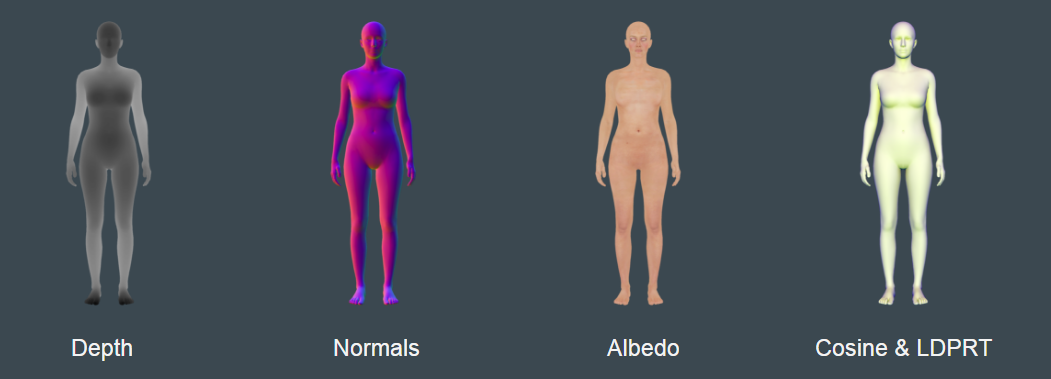
We use many different types of textures to describe the material of an object. I’ll discuss here mainly albedo maps and normal maps, but there are many others: specular maps, roughness maps, elevation maps, decals, and so on. Some are specific to a particular renderer.

Albedo maps show the diffuse colour of an object, the c_diff in equation (2). There’s no colour in absence of light, so albedo maps are in fact lit, but by a constant illuminant. Sometimes the albedo map contains some embedded shadows that come from ambient occlusion. This can help improving realism in real-time renderers, but it’s generally incorrect, because the colour of the ambient light will be wrong. If you see some funny shadows that you can’t explain, inspect the albedo maps.

Another important thing is that albedo maps need to be in linear RGB space. When images are displayed on screen, gamma correction needs to be applied to them. If you have only 8 bits to store luminance, 256 values will not be enough for the darks, since our eyes are very sensitive to changes in dark shades. Without increasing the number of levels, you would see the banding artefacts we discussed earlier. But we can apply a non-linear transform and store the pixels of the image in gamma space. If images are 8 bits, this is going to be always the case, but then the renderer will be responsible of converting the image to linear space before using it, because irradiance is only additive provided that everything is in linear space. If a material looks too bright, it could be that the albedo was saved in linear RGB but the renderer is mistakenly undoing the gamma. In the opposite mistake, the albedo could look too dark. All the problems with colour spaces also apply.

The albedo map in the right image is saved in linear RGB. Both albedos are previewed correctly in macOS because it knows how to interpret the colour profile, but V-Ray is applying the inverse gamma when it shouldn’t, resulting in a dark coat.

Normal maps describe the normal direction of a surface. What in normal jargon we’d call the “texture” of a piece of cloth, mostly refers to what normal maps are responsible of. A flat T-shirt is not really flat. You can see the depth of the threads if you look closely. Given enough computer power we could scan the exact geometry and use it as it is, without need of normal maps. But what we do to save resources is scan a tiny piece, and “bake” that geometry into a normal map, so we know how light will behave at a certain pixel, without needing to store all the exact geometry. If the normal map is missing, renders will lack “texture”, because light will look flat and boring.

When the normal map is missing, materials lack “texture” because light acts as if the surface was flat.

If you go back to the light equation, notice how the normal influences every light term, either diffuse or specular. Here’s an example of a purely diffuse material and the effect of the normal map on it:

The left image has no normal maps. The right image has a normal map. The shade it produces introduces depth to the material.

Environment maps

Environment maps are a special type of texture used to cheat a bit with lights. Textures in previous section were things applied to the object material, but environment maps are a substitute for lights. You capture a 360-degree image (or rather, 4π steradians, the whole sphere) in multiple exposures, and then you combine them into a single HDR map. After that, the software applies an integral over it to obtain an irradiance map (it looks like a blurred version of the image). If you want to know the irradiance value from a certain direction, you can simply sample the irradiance map. For specular reflections, you can directly sample the image.

Screenshot of HDRI Haven website, where you can find plenty of HDRI maps under Creative Commons license.

As mentioned earlier, if you notice lack of contrast in your image, it could be that your light source is not bright enough. If you are using an environment map, that means you didn’t capture enough exposure and your light just saturated to a bright spot. If you try to fix that afterwards by applying some gamma curve to the image, you may fix the contrast, but you may start experiencing banding artefacts at different luminance values.

Again, all the problems that we already mentioned at the beginning about colour spaces and image encoding apply here as well. Be very careful with your environment map, because if you get this wrong, all the lighting will be wrong, and it will be hard to decouple from all the other issues we have already mentioned. If you aren’t sure if the funny colours are due to materials or lights, try rendering white objects with that light, and also try replacing your light with some well known outdoors and indoors settings, and then look how the materials in your object look like.

Conclusion

This has been a long journey backwards. Quite thorough, but not complete. Follow the bibliography and links for more details. I hope that by reading this guide and by looking at the examples, people can start to classify different kinds of errors in renders and troubleshoot where necessary. To summarise:

first make sure you are communicating properly and that you use a common vocabulary;
make sure everyone involved has some means to see the same image, even if that means using a smartphone screen;
make sure images are saved in the correct format and with the correct colour space;
make sure the ray-tracer has the correct quality settings;
make sure there are no textures missing in the materials used in the 3D scene, and that those textures have also been created following the criteria above;
make sure your light covers the range of luminance it’s supposed to, and that it has the right colour.

And rest your eyes from time to time!

References

[1] Richard D. Zakia. Perception & Imaging. Focal Press, 2nd edition, 2002.

[2] Tom Stafford, Matt Webb. Mind Hacks, Tips & Tools for Using Your Brain. O’Reilly, 2005.

[3] Tomas Akenine-Möller, Eric Haines, Naty Hoffman. Real-Time Rendering, Third Edition. A K Peters, 2008.

Introduction to Skinning and 3D Animation

June 17, 2019 by David Gavilan·0 Comments

About 3D Animation

An animation is just a description of changes along a timeline. For a 3D object, there are mainly three ways of transforming its triangle mesh to create an animation:

Animation through affine transforms, which are usually rigid. With rigid transforms we can move or rotate a character. With a more generic affine transform, we can also scale the character up or down. See examples below.
Affine transforms
Animation through skeletons, attached to the character. The rigid transforms (sometimes with scaling as well) are applied per limb. We will introduce the concept of skinning later on, key to understand how this works.
Skeletal transforms
Animation through morphing of the mesh, that is, moving each vertex of the mesh separately and store its new location, or by describing its change through special functions. In 3D modelling software like Maya, you can create these morphs using something called Blend Shapes. Check this tutorial: How to animate a character using Blend Shapes. At Metail, we morph our avatars based on a parametric model we train from a database of thousands of real scans of people, so our morphs are described in terms of eigenvectors.
Character morphing

An animation file simply stores the different transformations for a few keyframes. You can think of a keyframe as a snapshot of time. For instance, at time 0 I’m standing, and at time 1 second I’m starting to kneel down. 2 seconds later I might be fully sat down. When the animation plays we simply interpolate transforms to figure out the position of things between those keyframes.

In this blog post we will focus on skeletal animation. For that, we will review the concept of space transforms, and then introduce skinning, the main tool for transforming a mesh with a skeleton.

Space transforms

In a previous blog post, we briefly reviewed how rendering works and posted a figure to summarize all the spatial transforms that get applied to a 3D object before it gets rendered on screen. Here’s the same figure, with an additional extra step to compute joint transforms in what we can refer to as the joint space:

Space and Joint Transforms

A transform in 3D is usually represented by a 4×4 matrix, which contains just scaling, rotation, and translation, until reaching the clip space. The clip space represents what the camera sees, so that transform matrix contains a perspective transform as well. The result gets normalized to a unit cube. If you convert the horizontal (x) and vertical axis (y) of that unit cube to pixel coordinates, you land in screen space, which it’s basically what you see on screen.

As an example, let us imagine an animator working on the next Antman movie. You can think of the animator as a puppeteer who:

moves Antman’s limbs to put him in a certain pose (in joint space);
repeats that process for several keyframes of an animation, be it walking or flying;
if Antman now needs to become tiny, we can just apply a scaling transformation in model space to reduce the size of the animated character;
to finally place Antman on top of a cupcake in a kitchen scene.

The director will place a camera looking at Antman, and all the transforms will finally be applied and the triangles will be rendered on screen. The renderer only needs to multiply each vertex of every object by each transform matrix in order to obtain the final vertex position on screen.

Skeleton creation

Rigging

Skeletons are usually created by an artist in a process known as rigging. A rig is just a series of connected joints used to describe animation. You can think of a joint as an anchor point placed around a bending or twisting point in the body, for instance, an elbow. Because the rig describes a hierarchy of joints through their connections, a joint inherits the transforms of their parents. So if you twist your thigh to the right, your foot will point to the right.

Rigging of a mesh

A very basic rig or skeleton just contains joint locations and the hierarchy, but you can also have orientation, which can be useful to represent twists of limbs along the correct axis. More often than not, we use the term bone interchangeably with the term joint. That is because, as we will see in the skinning section, either way we will just need a single matrix per joint or bone to compute the final vertex position. But in 3D modelling software, usually the bone is not just a transform matrix, but the structure that connects two joints. So if you have a joint in your shoulder, and another joint in the elbow, the shoulder bone is what connects the shoulder to the elbow. Therefore, you can describe bones in terms of starting position, length, and rotation.

What’s a good rig?

There is no single way to rig an object. The illustration below shows possible rigs for a sphere.

Rigs of a sphere

These are all “good” rigs, depending on the type of animation we are targeting. For instance, if we want to create the animation of a blob moving forward, any of the two first rigs could be used. The second one splits the body in left and right, so the blob could first move one side of the body and then the other. The third rig looks like the skeleton of a person. That means we could create the animation of a person targeted to that sphere. If we had a walking animation, it would look like a person is inside the blob and trying to move forward.

Notice that the joints don’t need to be inside the body. The last example above could be used to model a moving blob that looks as an starfish. The joints can be thoughts as strings that pull the mesh from the outside.

Weight painting

Up to this point, nothing will move on screen. The rig is used to conceptually define how we would like things to be posed or animated later on. But in order for the object to actually change, the artist needs to paint each vertex of the mesh with a weight. The weight is a number from 0 to 1 associated to a particular joint. You can have more than 1 weight per vertex, and the sum of all them must be equal to one. What it’s saying is how much each joint contributes or affects each vertex. For the previous sphere example, we could paint the sphere in different ways:

Weight painting of a sphere

In the first 2 examples, if you pull the joint associated with the red area, only that red area will move. If you pull both joints in opposite directions, your sphere will stretch like dough.

Weight paints are usually represented as heat maps in 3D modelling software. When you select a joint in weight-painting mode, you will see in red the vertices that have 1 as weight for that joint, and blue where the weight is 0. Below you can see an example of the arm of one of our avatars:

Vertex weights of a shoulder

In the example, I have selected the shoulder joint. Since it’s all red, the upper arm is only affected by changes to this joint. However, the armpit appears green because it’s not only affected by changes to the shoulder joint, but also by the transform of the collar joint. Notice that if I bend the shoulder, the forearm will move as well, even though it appears blue (weights equal zero). This is because the elbow joint inherits the transforms from the shoulder joint, as explained earlier. The vertices of the forearm need to be associated with the elbow joint only (forearm bone).

Skinning

Linear blending

Skinning, also known as vertex blending, enveloping, or skeleton-subspace deformation, is the process of transforming the mesh vertex positions according to the rig we created earlier. The most common skinning equation is the linear blending described below:

Skinning equation

Each vertex of the mesh is transformed to joint space, through the bind matrix. Then, you apply the joint transform for that particular point in time. That should convert back to model space. You apply the weight for that joint, and sum up the same operation for all the joints that affect that given vertex. (I’m using the same nomenclature as in Real Time Rendering, 3rd. Edition, by T. Akenine-Möller et al.)

Here’s a example of bending and twisting of the arm I showed earlier:

Bend and twist of an arm

Skinning artifacts

The linear blending equation does not care about the preservation of volume. It simply interpolates new vertex positions based on a weighted sum. That means that if you bend a shoulder too much, the area close to the joint may appear as a bulge:

Bulging artifact

Similarly, if you twist the shoulder too much, you will end up creating what it’s usually known as a candy-wrapper artifact:

Candy-wrapper artifact

There are alternatives to linear vertex blending to address those issues. Check SIGGRAPH 2014 course, Skinning: Real-time Shape Deformation. One of the alternatives is using dual quaternions. Here’s an illustration from that SIGGRAPH course:

Skinning using dual quaternions

Fixing artifacts with extra joints

Another common approach to address skinning artifacts is by adding extra joints, so we can split rotations across joints. For instance, if we want to twist the forearm by 180 degrees, we could add an extra joint between the elbow and the wrist, and split the twist between the two. The elbow joint could twist 90 degrees, and the middle of the forearm could twist another 90 degrees, so by the time we reach the hand we would have twisted it by 180 degrees already. See illustration below.

Forearm twist with extra joint

You have to be careful with these extra joints. The one I described above is meant to be used for twisting only. We can bend our arms from the elbow, but not from the middle of the forearm. If you use those for bending, you can create arms that look like rubber arms. See below.

Bending a twist-only joint

Resources

Apart from 3D modelling software like Maya (by Autodesk) or Blender (Open Source), I recommend taking a look at Adobe’s mixamo – it’s a web service that allows you to upload a mesh (a humanoid), which it then auto rigs for you. There are a couple of skeletons to choose from, and the software will automatically skin the mesh for you (assign proper weights). You can also try out many parameterized animations from the same site.

mixamo screenshot

The skinning equation is quite simple, so it’s not complicated to implement it yourself. I created a WebGL-based Model Viewer that lets you view the keyframes in an animation. I’ve continued its development here at Metail so we could do things like visualizing all the skinning weights simultaneously, instead of using a heatmap per joint. The output looks like this,

All the skinning weights at once

This is important for us so we can see where the boundary of the different skinning regions end up being for any arbitrary body shape that we create.

Summary

Skeletal animation is just an extra spatial transformation step in your rendering pipeline. Mathematically, it’s just more matrix multiplications to move from one space to another. In an animation, these matrices will change over time. However, the creation of good animations involves an artistic process that doesn’t necessarily correspond to real human anatomy. For instance, in order to prevent things like the candy-wrapper artifacts, we may introduce extra joints in our skeleton to distribute twists.

At Metail we create 3D avatars of arbitrary body shapes, morphed based on a mathematical model that uses the user tape measurements as an input. The resulting avatar has a skeleton that can be posed. You can, indeed, switch between a couple of poses in our live system. Avatars are posed using the skinning method discussed here. You can try it out at trymetail.com.

Introduction to Colour Spaces and DCI-P3

December 13, 2018 by David Gavilan·4 Comments

Introduction

I’ve always loved colour, and I’ve always been a bit geeky about it. Other kids would argue about football, but in my circle we’d go: “my Amiga 500 has 4096 colours, and yours has only 16”. And we counted the days for those 4096 to become 262144. But colour is not just numbers. And when now someone sends me an RGB triplet saying, “this colour: 146, 27, 98”, my brain just short-circuits. That’s not a colour, and I’ll explain why later. Colour and colour spaces are hard topics, and the more you dig into them, the more complex it gets, and the uglier the truth becomes.

Some of the topics around colour, like colour perception in humans, are still hot areas of research. They sometimes even become mainstream discussions in bars, like the white/orange dress meme a couple of years ago. But I won’t talk about colour perception today.

Instead, I will focus on a less mainstream but more technical topic, which is sadly neglected more often than I’d like: colour spaces. I’ll try to summarize the different concepts around colour spaces as briefly as I can, and then talk about a particular colour space that you may want to start using in your mobile apps: the Display P3 colour space.

Why do we see colour?

I’m not going to define what colour is. You probably know what it is even without a formal definition. Instead, I think it’s more useful to explain how colour is created.

We see colour because our eyes have photoreceptor cells, sensitive to different wavelengths of light. These photoreceptors are rods and cones in mammalian eyes, and ommatidia in arthropods. Although photoreceptors themselves do not signal colour, but only the presence of light in the visual field, the signals from the cones are used by the visual system to work out the colour. Here’s a figure of human photoreceptor absorbances for different wavelengths,

(Source: Wikipedia)

In terms of number of photoreceptors, you can say you see more colours than your cat does (they discern at least 3 or 4 colours), but a mantis shrimp sees many more colours than you (they have 16 types of cones). But also, the colours that you see may not be exactly the same I see. And it is also worth mentioning that luminance is orthogonal to colour, so a cat can see much better in the dark than we do.

Colour Spaces and Colour Models

These two terms get messed up together more often than not. A Colour Space organizes colours so they are reproducible in physical devices (e.g. sRGB, Adobe RGB, CIE 1931 XYZ), whereas a Colour Model is an abstract mathematical model describing the way colours can be represented as tuples of numbers (e.g. RGB, CMYK).

That distinction is really important. I often hear people telling each other random RGB tuples to communicate colours, and I have to assume those tuples are in sRGB colour space, with the gamma already applied. But even the gamma may change from system to system, so those numeric values really don’t tell me anything unless you specify a colour profile as well.

Another very important thing to remember is that there’s no single RGB colour space! Although in most desktop applications we use sRGB, cameras may use Adobe RGB because they need a wider gamut.

XYZ Colour Space and Colour Conversions

XYZ Colour Space is a device-invariant representation of colour. It uses primary colours that aren’t real, i.e., that can’t be generated in any light spectrum. That means we can even represent “imaginary colours”, that is, colours with no physical reality.

In XYZ, Y is the luminance, Z is the blue stimulation, and X is a linear mix. It is also very common to normalize this space by the luminance to obtain the xyY colour space. You may have seen the typical horseshoe shape from the xy chromacity space before,

CIE 1931 xy chromaticity space

The horseshoe shape is the gamut of human vision, that is, the colours that we can see. The curved edge is the spectral locus and represents monochromatic light, in nanometres. Notice that the straight line at the bottom, or line of purples, are colours that can’t be represented by monochromatic light. Read about CIE 1931 Colour Space to find more details.

The important thing to remember is that these diagrams are useful to visualize the gamut of different devices and the colour conversions that happen between them. For instance, in the example below, the green dot from an Adobe RGB Camera needs to be flattened down to a more yellowish green in order to be displayed in a laptop display. Note that in an RGB colour model, both values may look identical, e.g. (0, 255, 0), but they aren’t the same. This conversion may be irreversible if we aren’t careful. When printing this green, we want to go back to the closest match between the original green colour, and the greens that the printer can represent, not the yellowish green from the display.

(The image above is taken from Best Practices for Color Management in OS X and iOS, another recommended read.)

DCI-P3 Colour Space

The most common colour space for displays is sRGB. However, recent OLED displays have a wider gamut, so we need a better colour space to make the most out of them. DCI-P3 is a wide gamut RGB colour space. Apple calls it Display P3. Because the gamut is wider, you will need at least 16-bit per channel in order to store colours in P3. So if you are storing values as integers, instead of having maximum values of 255 per colour channel, now it will be 65535.

In order to visualize the differences between P3 and sRGB, I recommend using Apple’s ColorSync utility, which comes with macOS. This tool also has great colour calculators included that will help you understand all the different concepts from this blog post. It’s very simple to create a visualisation like the one below using that tool. This figure compares P3 and sRGB gamuts, plotted in L*a*b* colour space (close to human perception).

P3 vs sRGB in L*a*b* plot

Apple recommends the use of Display P3 for newer devices in its Human Interface Guidelines, so if you are developing a website or an app for iOS and/or macOS, it’s worth updating your authoring pipeline to use wide colour in every stage.

Most of MacOS and iOS SDK supports Display P3 already, with the exception of some frameworks like SpriteKit. The UIColor class has an initializer for displayP3. If you need to do the conversion yourself, I’ve written a couple of posts on how to compute (Exploring Display P3) and test (Stack Overflow). It boils down to this matrix that you can apply to your linear RGB colours (before applying the gamma) to convert from P3 to sRGB,

 1.2249  -0.2247  0
-0.0420   1.0419  0
-0.0197  -0.0786  1.0979

I’ve written a battery of colour conversion unit tests here: Colour Tests.

How much wider DCI-P3 is?

According to Wikipedia, the DCI-P3 colour gamut is 25% larger than sRGB. According to my accounts, it’s approximately 39% bigger. I’ve counted all the 24-bit samples in linear Display P3 RGB (16M) that fall out of sRGB, and that accounts for approximately 4.5M (~28%).

I’ve also tried visualising these differences in different ways. I ended up creating an iOS app, Palettist, to help me create colour palettes with P3 colours that fall outside the sRGB gamut. The result is some discrete palettes where each square is in P3, and a circle inside it with the same colour clamped to sRGB. Here’s one of such palettes,

DisplayP3-only Palette

Depending on where you are reading this, you may or may not see the circles. More details in this blog post: Display P3 vs sRGB. If you have a modern iOS device, try downloading this palette, and uploading it to, say, Instagram. You will see the circles, but the moment you click “Next”, all colours will look duller and the circles will disappear (you don’t need to actually post it; Instagram converts it to sRGB before uploading). Please try to use these palettes to test if an app supports P3 or not.

Rendering intent

If you see circles in the colour palette I posted above, but you are sure your display is sRGB, it could be that the colour management in your OS is trying its best by applying a rendering intent before displaying the image. The common modes are these two:

Relative Colorimetric intent: clamp values out of gamut to the nearest colour. This causes posterization (you won’t see the circles).
Perceptual intent: blindly squash the gamut of the image to fit the target colour space. This reduces saturation & colour vibrancy (but you’ll see the circles). We say “blindly” because even if it’s just one pixel that’s out of gamut, it will cause the whole image to shift colour… The amount of compression will be shown in the ICC profile

There are other modes, like Absolute Colorimetric intent and Saturation intent. Check this article for details: Understanding Rendering Intents.

A note about gamma

Gamma correction alone deserves a separate blog post… But it’s important to emphasize here that when people give you an RGB triplet like (181, 126, 220) (Lavender), not only do they mean it’s in sRGB (and there are different sRGB profiles), but also they mean the gamma correction – an exponential function – has already been applied. If you do your own colour conversions with the CIE Colour Calculator, you also need to remember that the sRGB illuminant is D65, but it’s encoded with D50.

Why do we apply gamma? This is because equal steps in encoded luminance correspond roughly to subjectively equal steps in brightness. Read Gamma Correction.

If you only have 8 bits to store a luminance value, you better store it with the gamma applied, so you lose less perception-valuable information. However, if you are into 3D graphics, remember that light computations should happen in linear space!

The final decision: choosing a colour space

This is my small personal guide to choosing a colour space, depending on the occasion:

L*a*b* for Machine Learning, because the Euclidean distance between 2 colours in L*a*b* is closer to perceptual distances.
RGB colour spaces
- Linear RGB if you are working with light (3D graphics), because light can be added linearly;
- DCI-P3 if you target newer screens, because you can represent more colours; sRGB if you can only afford 8-bit per channel – make sure the gamma is applied to avoid banding artefacts in dark colours (the eye is more sensitive to differences in dark areas)

For the colour model,

RGB, if you are doing light or alpha blending computations, you better stick to RGB;
HSV for design, because the representation is intuitive; and if you are colour-blind, you can adjust saturation and luminance without worrying about accidentally having changed the hue.

Summary

Thanks for reading this long blog post! To be brief, I’ve tried to summarize it all with a few bullet points:

Cats may dream in colour
Every human is unique
Colour Space ≠ Colour Model
Display-P3 > sRGB
ColorSync Utility is your friend
Use provided P3 palettes as reference
Choose appropriate Colour Space & Gamma for the occasion (storage, ML, 3D)

From Consumer Products to Internal Tools

August 29, 2018 by Rich Taylor·0 Comments

It’s sometimes necessary for an organisation to develop software to support its internal operations. Doing this well is less straightforward than one might think. In this post, I examine some of the challenges faced by product teams building internal tools, and share some lessons learned from working on consumer products that are applicable in overcoming them.

The value that comes from using a tool is in how it improves a process. When an actor from a user story hacks around the current process to get their job done, it’s a good indicator that a new tool might be needed. Another step may be required in the workflow, for instance, if users frequently open another browser window to perform a particular task. There are also situations when a new feature is required for reasons other than improving the user experience. We may wish to gather data to train a machine learning algorithm which will ultimately allow us to automate a manual process.

Another reason to build our own tools is to avoid vendor lock-in – the situation where we become unable to switch our process from one product or service to another without substantial costs. However, it’s important to remember, that the decision to adopt any technology, be it proprietary or open source, is a long term commitment. While there are compelling reasons to choose an open source solution, we may incur large costs in adapting it to fit our process or in simply learning how to use it well if the base technology and expertise doesn’t already exist in our stack.

How do we avoid reinventing an existing tool which already fits our purpose? Cast a wide net to find out whether or not a cost-effective solution is already available on the market. Don’t hesitate to open this investigation to the operations and engineering teams. Their involvement is important; although they may have a good understanding of the problem domain, they often lack the marketplace visibility and exposure to product demos or sales-driven trials that product managers or the business team have. How have stakeholders solved similar problems at previous organisations? Getting input from every player at this stage can eliminate a lot of uncertainty around the necessity of the work involved.

When there’s a genuine need for a bespoke solution because the marketplace doesn’t offer an essential feature, expectations may still be high because users will be familiar with similar well established, high quality software. We can manage these expectations by including metrics and benchmarking on the product roadmap and by building them into the product as early as the size of the user base justifies the effort. This also gives us the confidence to abandon our developing solution for something better if it isn’t performing as we’d hoped. Involving users in the development cycle early can also help – users are more forgiving of work in progress when they are part of its inception and growth.

We can develop the best understanding of our customers’ pains by beginning the development cycle with an exploratory research phase. This allows us to get to the root of the problem and discourages us from rushing to a suboptimal solution. IDEO’s human centered design framework provides some useful techniques for doing this, such as by having customers map their journey through the process or by observing the journey directly, taking note of any unnecessary cognitive overhead and the behaviours of our “power users”.

The research phase may also take the form of a design sprint, where inexpensive prototype solutions are validated by observing how customers interact with them. Be sure to meet with every possible user at this stage. Not only will users at different levels in the workstream be concerned with different tasks; they may also have different working styles which the UX will need to accommodate. This can seem like a large upfront time investment, but it’s far less costly than waiting until after UAT to learn that the chosen solution doesn’t meet the customers’ needs.

What do we do when we don’t have the luxury of conducting a lengthy exploratory research phase? When pivoting, a startup or a product team needs to adapt its operations at short notice, sometimes resulting in the prioritisation of a completely new set of features. As an internal product team, our colleagues are our customers; we should therefore be well positioned to meet with them early and often. When we don’t, we develop false assumptions about where the process bottlenecks are. When gathering requirements, don’t be afraid of asking “why” too often. On first asking, our customers might tell us what they think we want to hear, suggesting “quick wins” or solutions they believe are easy to pull off, rather than revealing their greatest pains. Persistence in our questioning will pay dividends.

Feature requests are, in theory, better supported by an internal development team than an outsourced one, and straightforward for us to act on because we can easily seek clarification. In practice, we need to consider the long term costs of maintaining these features. Even simple estimation exercises like Josh Pigford’s build vs. buy calculator can be of help. More often than we’d like, resource constraints may mean that we’re not able to balance the local needs of our internal customer with the overall needs of the business. When that’s the case, it’s important for the health of the relationship to communicate why the work can’t be done at this time. Shared understanding and goals reduces the tension between the team and encourages us to review and update these priorities continuously.

If our tool doesn’t require expertise to operate, then we’re able to easily dog food our product across the organisation. This lets us find and form relationships with product-minded users who can identify problems which we may have become blind to when designing and building. Take advantage of this, remembering that the managers of most consumer products don’t have this luxury! Developing these relationships by holding “open office hours” increases the quality and quantity of feedback we receive.

Once the tool has been built, how do we ensure that product development continues smoothly? Having the development team focus early on the infrastructure necessary to support continuous delivery allows us to launch and begin gathering feedback as early as possible and keep a tight, iterative development cycle. when done well, we can reap the same benefits from practicing agile with our internal tool development as with our consumer products. MVPs are a great way to accelerate learning, but we shouldn’t be duped into thinking that it’s acceptable to produce sub-standard features, believing that they can be “improved incrementally” because we have only our colleagues’ expectations to manage. The launched product should consist of the minimum set of features required to deliver value, but each of those features needs to meet some previously agreed standards.

When planning, it’s important to be mindful of how our users will onboard. We’re familiar with the notion that “good design needs no instructions”, but even refined technical operational processes require some training. To save time and effort, training for our tools could take the form of a webinar which can be made available online for later access. Announcing the initial launch internally and continuing to meet frequently with customers can both help drive adoption, and announcing subsequent feature releases can help users imprint on workflows. Make all of the feedback received easily accessible to engineers, for example, through a dedicated Slack channel or integration. Above all, celebrate as a team when users are delighted.

In summary, it’s easy for us to become complacent or misguided when we’re designing for our colleagues. We know their organisation, its mission and its roadmap. We know their titles, respective roles and working environment. We may therefore assume that we know what’s best for them, and worse, we won’t make the time to validate those assumptions. Instead, if we do our internal customers the same courtesies as we would our flagship product users, but acknowledge when to treat them differently, we stand a much better chance of delivering the best possible outcome.

Skin colour authoring using WebGL

June 28, 2018 by David Gavilan·1 Comment

About skin colour authoring

Part of our MeModel development process involves skin colour matching. We have to match our 3D avatars to a photographic reference. We have attempted to do this automatically in the past, but as the lighting process became more complex, the results were no longer good and it required a lot of manual tweaking. In effect, we needed to manually author the skin colour, but writing parameters by hand and trying them out one at a time is a tedious process. That’s why we decided to create an interactive tool so we could see the result immediately and iterate quickly.

The first choice we made was the platform: the browser. If we wrote this tool for the web, then we could share it immediately with remote teams. It’s a zero-install process, and therefore painless for the user.

We wrote a prototype that would use a high-resolution 2D canvas, and transform all the pixels in simple for-each loops. However, this was far from interactive. For our images, it could take a couple of seconds per transform, not very pleasant when adjusting parameters with sliders. You could try to parallelise those pixel loops using Javascript workers, for a 2 or 3-fold speed increase. But the real beast for local parallel processing is your GPU, giving us in this case more than a 100-fold speed increase.

So we decided to make the canvas a WebGL canvas. WebGL gives you access to the GPU in your machine, and you can write small programs for it to manipulate all pixels of the image in parallel.

Quick introduction to rendering

Forward rendering

The traditional programmable rendering pipeline is something that in the computer graphics jargon is referred to as forward rendering. Here’s a visual summary,

Forward rendering pipeline

Before you can render anything, you need to prepare some data buffers with your vertex positions and any parameters you may need, which are referred to as uniforms. These buffers need to be in an area of memory that your GPU can access. Depending on your hardware, that area could be the same as the main memory, or a separate graphics memory. WebGL, based on OpenGL ES 2.0 API, has a series of functions to prepare this data.

Once you have the data ready, then you have to provide two programs to the GPU, a vertex shader and a fragment shader. In OpenGL/WebGL, these programs are written in GLSL, and compiled during run time. Your vertex shader will compute the final position and colour of your vertices. The GPU will rasterize the vertices for you (this part is not programmable), which is the process of computing which pixels the given geometry will cover. Then, your fragment shader program will be used to decide the final pixel colour on screen. Notice that all the processing in both the vertex and pixel/fragment shaders is done in parallel, so we write programs that know how to handle one data point. There’s no need to write loops in your program to apply the same function to all the input data.

A traditional vertex shader

There are basically two things that we compute in the vertex shader:

Space transforms. This is how we find the position of each pixel on screen. It’s just a series of matrix multiplications to change the coordinate system. We pass these matrices as uniforms.
Lighting computations. This is to figure out the colour of each vertex. Assuming that we are using a linear colour space, it is safe to assume that, given 2 vertices, the interpolation of pixel colours that happens during rasterization is correct because irradiance is additive.

A traditional vertex shader

Both the space transforms and lighting computations can be expensive to compute, so we prefer doing it per vertex, not per pixel, because there are usually fewer vertices than pixels. The problem is that the more lights you try to render, the more expensive it gets. Also, there’s a limit of the number of uniforms you can send to the GPU. One solution to these issues is deferred rendering.

Deferred rendering

The idea of deferred rendering is simple: let’s defer the lighting & shading computation until a later stage. It can be summarized with this diagram,

Deferred rendering pipeline

Our vertex shader will still compute the final position of each vertex, but it won’t do any lighting computation. Instead, we will output any data that will be needed for lighting later on. That’s usually just the depth (distance from the camera) of each pixel, and the normal vectors. If necessary, we can reconstruct the full 3D position of each pixel in the image, given its depth and its screen coordinates.

As I mentioned earlier, irradiance is additive. So now we can have a texture or a buffer where to store the final irradiance value, and just loop through all the lights in the scene and keep summing the pixel values in the final texture.

Skin colour authoring tool

If you followed so far, you may see where this is going. I introduced deferred rendering as the process of deferring lighting computation to a later stage. In fact, that later stage can be done in a different machine if you wanted to. And that’s precisely what we have done. Our rendering server does all the vertex processing, and produces renders of the albedo, normals, and some other things that we’ll need for lighting. Those images will be retrieved by our WebGL application, and it will do all the lighting in a pixel shader. The renders we generate look like this,

MeModel GBuffer

Having these images generated by our server, the client needs to worry only about lighting equations, and we only need a series of sliders that connect directly to the uniforms we send to the shader to produce a very responsive and interactive tool to help us author the skin tones. Here’s a short video of the tool in action,

The tool is just about 1000 lines of pure Javascript, and just 50 lines of shader code. There are some code details in the slides here:

Metail Skin Colour Authoring Tool from David Gavil

(These slides were presented in the Cambridge Javascript meetup)

Summary

Javascript & WebGL are great for any graphic tool (not only 3D!): being in the web means zero-install, and being in WebGL should mean it gives you interactive speeds. Also, to simplify the code of your client, remember that you don’t need to do all the rendering in the client. Just defer the things that need interaction (lighting in our case).

“You need Terry on your project? Ok, here’s what you need to know…”

June 12, 2018 by Nick Maidment·0 Comments

Sometimes people move teams. The reasons why can be varied. It could be this person’s skills are needed on a different set of work. Or maybe to drive their personal development you need to provide other opportunities for them. Or perhaps they are unhappy for some reason. Generally speaking it’s pretty healthy for a business to move people about. But regardless of the reason, it’s going to affect your organisation. By changing someone’s line management and transferring a person between teams you are changing the team dynamics of two teams. In order to help keep both the teams and that individual happy, you really need to understand what makes them tick.

If you’re the manager who is losing a person, you hopefully already have a working relationship with them but you may not have had the head space to figure out how this is going to affect your team. If you’re the manager that is receiving a new team member, you might already have a fair idea of what your team needs but you may not know the person that is joining you.

Depending on your organisation, the hand over of line management may happen casually between two managers, with little to no structure. When I looked online, I couldn’t really see anything to help this transition. At the very least you should have a conversation with the line manager who is giving up or receiving the line report. Before you have the meeting, try to summarize (in writing) what the reasons for the move are. It’s good for everyone involved to be on the same page.

For the process of handing over itself, I came up with a few questions you can ask or answer to ease the movement of people around the organisation.

Happiness

What motivates / demotivates this person?
Are they happy at work?
Who are their friends at work?
Do they have any triggers for things that upset them or that they have particularly strong opinions about?
Are there areas where they’ve been particularly happy or excited to work on in the past?

Communication

What are they like on a 1:1 basis?
What are they like in a group setting?
Have they raised any concerns or needs over the move?

Work/Life

How well do they manage their work / life balance?
What do they do in their free time? Any hobbies?
How is their general well-being (both home and work)?
What are their regular working hours/days?
Do they have any “invisible” commitments outside work that we need to ensure they’re supported with?

Personal Development

What personal goals are they working towards?
Do they want or need training on anything?
What was their biggest success recently?
Have they struggled with anything recently?
What are they hoping to get from the change?
Do they have an existing buddy/mentor/coach – will that relationship change if they move?

Support / Management

How do they prefer to be supported/managed?
Are there any current issues or problems that need managing?
What did they like / dislike about their old team?
What are their strengths and weaknesses?
Do they have any preferences/strengths/issues working with particular technologies or environments?
When are they going to move and sit with the new team?

You might not have, or be able to get all the answers to the questions, but finding out as much as you can will give you a head start in being able to build rapport with your new line report. It’ll also help you settle them in and set them on the path to building new relationships with other people in the team. Try it out the next time you have people coming or going from your team.

For more on Metail’s culture and team, please visit www.metail.com/careers

Brainstorming: Spark Ideas

April 2, 2018 by David Gavilan·0 Comments

While working in the games industry in Japan, I attended a seminar about brainstorming. The instructor, professor Hidenori Satō, has written dozens of books on the subject. Unfortunately for many of us it seems his work has not been translated from Japanese, so here’s a brief introduction to his approach. I’ve translated the method he introduced to us as “Spark Ideas” (スパーク発想法). At the beginning of his seminar Prof. Satō led in with the following quote attributed to Thomas Edison: “Genius is one percent inspiration and ninety-nine percent perspiration”. I read this in two ways: first, even if you have ideas, they mean nothing if you don’t put in sufficient effort to realize them; second, you may have a sudden bright idea once in a while, but to generate ideas continuously, you need to make an active effort – and probably use a tool like the one I describe here.

The brainstorming process

Often we try to think of ideas directly from a theme. Unless you’re in a moment of “inspiration” this is hard. For the “perspiration” moments, we need hints, like the one Newton got from an apple falling from a tree. The best way of getting these hints is by changing the Point of View. And that’s all you need to remember! (*^ω^*)

Brainstorming process

You can think of the Spark method as a “cheat sheet” with a series of keywords to help you get started with your brainstorming.

Points of View for Spark Ideas

Prof. Satō lists up 5 basic Points of View (PoV) to get started with the exercise:

State of affairs
Point of view of the other
Change character
Change case
Free of constraints

Working through these first five perspectives is usually enough, but there’s an extra list if you want to dig deeper:

Triple ease
Fun
Positivation
Indirection
3D expansion
Similar case
General case

I will describe all these points in detail later, but let’s jump first to how to do the exercise.

Brainstorming with the Spark Sheet

I recommend time-boxing the exercise. From experience, the “State of affairs” is usually the most important PoV, so expect to spend at least twice the time in that one as opposed to the others. If you need tons of ideas, you may want to attempt all 12 PoVs, though it may take too long. Even if you spend only 10 minutes per PoV, it will take at least 2 hours to finish.

If you are doing the exercise with enough people you may choose to divide them into groups. You could assign a couple of PoVs per group, with one group dedicated solely to “State of Affairs”.

Once you have allocated time, and appropriately divided people into groups, you just need paper or a whiteboard. Write the PoV and the theme on the top, and draw 3 columns. The first column are hints, that should come from the PoV. Write hints with as much detail as possible. The middle column will be for direct ideas, coming straight from the hints. These too should be as detailed as possible.

The third column is for ideas from association, things related to an idea from the middle column. These can be something that follows on in order from the initial idea, is the exact opposite of the idea, or just things that go together. It helps to have a cheat sheet with keywords on one side. Your sheet of paper will look like this:

Brainstorming example: Spark Sheet Pollution

Spark Sheet about Pollution

Keywords to get started

I’ve tried to select a few keywords for each PoV so you can get started.

(1) State of affairs

Status
1. Where are we at? Contents, outlook, flow, related work, schedule, place
2. Domain, level, quantity, season, important factors
Target
1. Characteristics, functionality, structure, processes, elements, type
2. Materials, size, weight, color, design, definition
Self
1. Company values, our technology, our resources, strengths & weaknesses
2. Budget, available developers, external opportunities
Main point
1. Reason for it, difficulties
2. Essential conditions

(2) PoV of the other

Target user(s), as detailed as possible
1. Adult A, kid B, high-school girl C, athlete, married person, old lady from the neighbourhood, a person with 2 dogs, etc.
Requests/needs, correct & detailed
1. Can we ask/have we asked users?
2. Person status, surroundings, circumstance, specialty, personality, real thinking, new thinking, needs, values, requests, dissatisfaction, worries, likes, opinions, feeling, goals, and conditions.

(3) Change character

Think of another person and write down their name.
How would they do things?
1. Way of thinking, behaviour, performance, personality, strengths
2. Ask them directly whenever possible!
Examples
1. Close person: colleague, boss, junior staff, from another team, related, from same industry, family member, friend, someone with similar/opposite interests, acquaintance, neighbour, professor, student of a higher/lower grade
2. Famous/historical: Buddha, Jesus, Bono, Björk, John Lennon, Messi, Trump, Picasso, Tom Daley, Tom Adeyoola, Tom Jones, Tom & Jerry
3. Role model: an expert, specialist, experienced person, aficionado, protagonist of a story/tale

(4) Change case

Think of the theme and target, and find a similar topic
Write down the contents (status, method, conditions) in detail
Examples
1. Direct method (visual): picture the theme in a broader sense, and give an example from intuition. E.g. “reduce stock” → “reduce ingredients”
2. Indirect method (logical): think of the essence of the theme, and from it give another example. E.g. “reduce stock” → “reduce unnecessary stuff” (essence) → “reduce flavour additives”
3. Close example (change from same class): e.g. “sell cameras” → “sell computers”
4. Far example (different class): e.g. “sell cameras” → “become famous” (sell brand)

(5) Free of constraints

Ideal
1. What is the state we want to be in? (in detail)
2. What’s the ideal, the best situation?
3. Write down the “ideals” as Hints, and how to realize/get close to those as Ideas.
Break norms
1. Try to break the rules: odd techniques, silly things, nonsensical, fancy, dream, insane, not common sense, innovation, daring
2. Write down as Ideas the way you’d get there.

Extra PoVs

Triple ease
1. Low-hanging fruit: do easy things first
2. Divide-and-conquer: divide in several parts, and assign to different people/teams
3. Reduction: reduce the quantity or targets. Make our lives easier.
Fun
1. Make it fun or interesting; add hobbies; gamify
Positivation
1. turn upside-down; take the negatives and turn them into positives;
2. find the positives and work on them
Indirection
1. Soften/cushion the blow;
2. Make it indirect; mediation
3D Expansion: think of these 3 dimensions
1. Space: expand the space, the area; change the place.
2. Time: expand time. Think of the future and the past. Think in a longer span.
3. Human: expand the human circle. Think of others. Get help from the crowd.
Similar case
1. Compare to similar cases
2. Compare with cases that offer contrast
General case
1. Remove the particular case. Look at the forest, not at the tree.
2. Think of the system

Rank the ideas

Once you’re done, you will end up with dozens of ideas. You may want to quickly eyeball the ones that lack detail or that are obviously flawed in some way and discard them to save time. Or you can focus on the ideas with many arrows coming to them. For the ideas you select to explore further, use a ranking mechanism, a simple example being the combination of impact and feasibility. For instance,

Theme: Do something about pollution — Best 3 ideas	Impact	Feasibility	Expectation (I×F)	Rank
Bring leaflets to schools	2	4	8	2
Gather signatures in online petition about cigarettes	3	2	6	3
Create a game where each stage is about a pollutant	3	4	12	1

Hopefully your Spark Sheets will be sufficiently detailed that they will also help you to start producing a plan for those selected ideas.

Conclusion

Generating novel ideas from nothing is a big challenge to some of us but a bit of structure in a brainstorming session can make a huge difference. If you’re stuck, try using a tool like this and be surprised at the volume of ideas your brains can produce. And as in so many other things, the more you practice the better you’ll get at it.